Command Line Tools
The command line interface to sotodlib is mostly convenience wrappers around high level functions in the package.
Hardware Configuration
There are several tools for simulating, selecting subsets from, and plotting hardware configurations. Currently the code writes hardware configuration data into the TOML format, which can represent basic scalar data types as well as lists and dictionaries. Under the hood it uses the python toml package. This format is simple to read and even edit manually (hopefully that will be a rare occurrence!). By default the dumping functions write this data in gzipped files and loading supports both gzipped and uncompressed TOML files.
Simulating
Until we have real hardware properties we can create a mock configuration with this script:
usage: so_hardware_sim [options] (use --help for details)

This program simulates the current nominal hardware model and dumps it to disk

optional arguments:
  -h, --help   show this help message and exit
  --out OUT    Name (without extensions) of the output hardware file
  --plain      Write plain text (without gzip compression)
  --overwrite  Overwrite any existing output file.
You can specify the output file root name (the toml and gz extensions will be added) and whether to overwrite any existing file by the same name.
Basic Info
You can dump very basic info about a hardware file with this tool:
usage: so_hardware_info [hardware file, [hardware_file]] ...

This program reads a hardware model and prints some summary text to the
terminal.

positional arguments:
  hardware    Input hardware file

optional arguments:
  -h, --help  show this help message and exit
If you need more details, you should just get an interactive python session and load the hardware model and explore it.
Selecting / Trimming Detectors
Starting with a large hardware model for the whole experiment, we usually want to select a subset of the detectors in order to do some analysis task. You can use this command line tool to read an existing hardware configuration, apply some selection, and dump out the result as a new configuration. Under the hood this just uses the sotodlib.hardware.Hardware.select() method.
usage: so_hardware_trim [options] (use --help for details)

This program reads a hardware model from disk, selects a subset of detectors,
and writes the new model out.

optional arguments:
  -h, --help            show this help message and exit
  --hardware HARDWARE   Input hardware file
  --out OUT             Name (without extensions) of the output hardware file
  --plain               Write plain text (without gzip compression)
  --overwrite           Overwrite any existing output file.
  --telescopes TELESCOPES
                        Select only detectors on these telescope (LAT, SAT0,
                        SAT1, etc) . This should be either a regex string or a
                        comma-separated list of names.
  --tubes TUBES         Select only detectors on these tubes. This should be
                        either a regex string or a comma-separated list of
                        names.
  --match [MATCH [MATCH ...]]
                        Specify one or more detector match criteria. Each
                        match should have the format '<property>:<regex or
                        list>'. The regex expression should be valid to pass
                        to the 're' module. If passing a list, this should be
                        comma-separated. For example, --match 'band:MF.*'
                        'wafer:25,26' 'pol:A'
Basically you can do a coarse selection by telescope or tube, as well as apply other selection criteria on the detector properties. See the example below.
Visualization
usage: so_hardware_plot [options] (use --help for details)

This program reads a hardware model and plots the detectors. Note that you
should pre-select detectors before passing a hardware model to this function.
See so_hardware_trim.

optional arguments:
  -h, --help           show this help message and exit
  --hardware HARDWARE  Input hardware file
  --out OUT            Name of the output PDF file.
  --width WIDTH        The width of the plot in degrees.
  --height HEIGHT      The height of the plot in degrees.
  --labels             Add pixel and polarization labels to the plot.
Example
Putting the previously discussed tools together, let’s make a plot of just detectors on SAT2 that are in wafers 33 and 38, in band MFS2, have “A” polarization (“A”/”B” are the 2 orthogonal polarizations), and which are in pixels 20-29 and 50-55. This is a very artificial selection, but demonstrates the use of the tools. First simulate the full hardware configuration:
%> so_hardware_sim --out hardware_all --overwrite

Getting example config...
Simulating detectors for telescope LAT...
Simulating detectors for telescope SAT0...
Simulating detectors for telescope SAT1...
Simulating detectors for telescope SAT2...
Simulating detectors for telescope SAT3...
Dumping config to hardware_all.toml.gz...
Although the output file is only a few MB, we can see it has a lot of stuff in there:
%> so_hardware_info hardware_all.toml.gz

Loading hardware file hardware_all.toml.gz...
cards       :    48 objects
    00, 01, 02, 03, 04, 05, 06, 07, 08, 09, 10, 11, 12, 13, 14, 15, 16, 17,
    18, 19, 20, 21, 22, 23, 24, 25, 26, 27, 28, 29, 30, 31, 32, 33, 34, 35,
    36, 37, 38, 39, 40, 41, 42, 43, 44, 45, 46, 47
crates      :     8 objects
    0, 1, 2, 3, 4, 5, 6, 7
bands       :     8 objects
    LF1, LF2, MFF1, MFF2, MFS1, MFS2, UHF1, UHF2
wafers      :    49 objects
    00, 01, 02, 03, 04, 05, 06, 07, 08, 09, 10, 11, 12, 13, 14, 15, 16, 17,
    18, 19, 20, 21, 22, 23, 24, 25, 26, 27, 28, 29, 30, 31, 32, 33, 34, 35,
    36, 37, 38, 39, 40, 41, 42, 43, 44, 45, 46, 47, 48
tubes       :    11 objects
    LT0, LT1, LT2, LT3, LT4, LT5, LT6, ST0, ST1, ST2, ST3
telescopes  :     5 objects
    LAT, SAT0, SAT1, SAT2, SAT3
detectors   : 66844 objects
    (Too many to print)
This is the kind of file that in the future could be versioned and be associated with a valid time range. It should really just be used as the starting input. First let’s trim out just the detectors on SAT2:
%> so_hardware_trim --hardware hardware_all.toml.gz \
   --out sat2 --overwrite \
   --telescopes SAT2

Loading hardware from hardware_all.toml.gz...
Selecting detectors from:
  telescopes = 'SAT2'
Dumping selected config to sat2.toml.gz...
This produces a file called “sat2.toml.gz”. This has only detectors on this telescope:
%> so_hardware_info sat2.toml.gz

Loading hardware file sat2.toml.gz...
cards       :     7 objects
    32, 36, 37, 34, 35, 38, 33
crates      :     2 objects
    5, 6
bands       :     2 objects
    MFS2, MFS1
tubes       :     1 objects
    ST2
telescopes  :     1 objects
    SAT2
wafers      :     7 objects
    32, 36, 37, 34, 35, 38, 33
detectors   : 11116 objects
    (Too many to print)
We can plot this as well:
%> so_hardware_plot --hardware sat2.toml.gz \
   --out sat2.pdf

Loading hardware file sat2.toml.gz...
Generating detector plot...
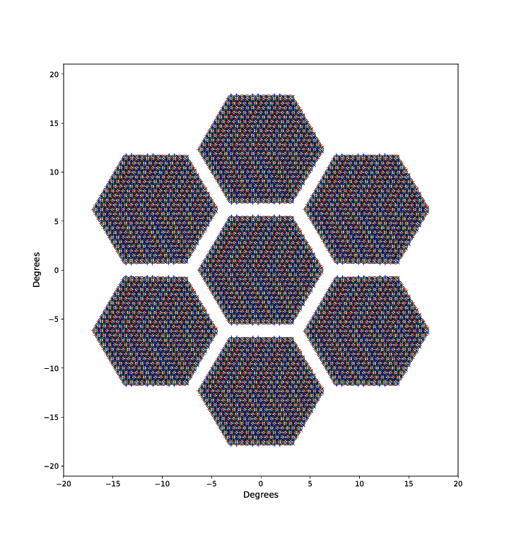
This outputs a PDF that you can “zoom in” to see details, but the image here is just a low-res PNG.
Back to our original selection goal. We can use lists of values to match detector properties or valid python regular expressions. We can trim out just those detectors with:
%> so_hardware_trim --hardware sat2.toml.gz \
   --out my_dets --overwrite --match \
   "wafer:33,38" \
   "band:MFS2" \
   "pol:A" \
   "pixel:(2.|5[0-5])"

Loading hardware from sat2.toml.gz...
Selecting detectors from:
  wafer = r'['33', '38']'
  band = r'MFS2'
  pol = r'A'
  pixel = r'(2.|5[0-5])'
Dumping selected config to my_dets.toml.gz...
Now explore this selection result:
%> so_hardware_info my_dets.toml.gz

Loading hardware file my_dets.toml.gz...
cards       :     2 objects
    38, 33
crates      :     2 objects
    6, 5
bands       :     2 objects
    MFS1, MFS2
tubes       :     1 objects
    ST2
telescopes  :     1 objects
    SAT2
wafers      :     2 objects
    38, 33
detectors   :   200 objects
    33_200_MFS2_A, 33_201_MFS2_A, 33_202_MFS2_A, 33_203_MFS2_A,
    33_204_MFS2_A, 33_205_MFS2_A, 33_206_MFS2_A, 33_207_MFS2_A,
    33_208_MFS2_A, 33_209_MFS2_A, 33_210_MFS2_A, 33_211_MFS2_A,
    33_212_MFS2_A, 33_213_MFS2_A, 33_214_MFS2_A, 33_215_MFS2_A,
    33_216_MFS2_A, 33_217_MFS2_A, 33_218_MFS2_A, 33_219_MFS2_A,
    33_220_MFS2_A, 33_221_MFS2_A, 33_222_MFS2_A, 33_223_MFS2_A,
    33_224_MFS2_A, 33_225_MFS2_A, 33_226_MFS2_A, 33_227_MFS2_A,
    33_228_MFS2_A, 33_229_MFS2_A, 33_230_MFS2_A, 33_231_MFS2_A,
    33_232_MFS2_A, 33_233_MFS2_A, 33_234_MFS2_A, 33_235_MFS2_A,
    33_236_MFS2_A, 33_237_MFS2_A, 33_238_MFS2_A, 33_239_MFS2_A,
    33_240_MFS2_A, 33_241_MFS2_A, 33_242_MFS2_A, 33_243_MFS2_A,
    33_244_MFS2_A, 33_245_MFS2_A, 33_246_MFS2_A, 33_247_MFS2_A,
    33_248_MFS2_A, 33_249_MFS2_A, 33_250_MFS2_A, 33_251_MFS2_A,
    33_252_MFS2_A, 33_253_MFS2_A, 33_254_MFS2_A, 33_255_MFS2_A,
    33_256_MFS2_A, 33_257_MFS2_A, 33_258_MFS2_A, 33_259_MFS2_A,
    33_260_MFS2_A, 33_261_MFS2_A, 33_262_MFS2_A, 33_263_MFS2_A,
    33_264_MFS2_A, 33_265_MFS2_A, 33_266_MFS2_A, 33_267_MFS2_A,
    33_268_MFS2_A, 33_269_MFS2_A, 33_270_MFS2_A, 33_271_MFS2_A,
    33_272_MFS2_A, 33_273_MFS2_A, 33_274_MFS2_A, 33_275_MFS2_A,
    33_276_MFS2_A, 33_277_MFS2_A, 33_278_MFS2_A, 33_279_MFS2_A,
    33_280_MFS2_A, 33_281_MFS2_A, 33_282_MFS2_A, 33_283_MFS2_A,
    33_284_MFS2_A, 33_285_MFS2_A, 33_286_MFS2_A, 33_287_MFS2_A,
    33_288_MFS2_A, 33_289_MFS2_A, 33_290_MFS2_A, 33_291_MFS2_A,
    33_292_MFS2_A, 33_293_MFS2_A, 33_294_MFS2_A, 33_295_MFS2_A,
    33_296_MFS2_A, 33_297_MFS2_A, 33_298_MFS2_A, 33_299_MFS2_A,
    38_200_MFS2_A, 38_201_MFS2_A, 38_202_MFS2_A, 38_203_MFS2_A,
    38_204_MFS2_A, 38_205_MFS2_A, 38_206_MFS2_A, 38_207_MFS2_A,
    38_208_MFS2_A, 38_209_MFS2_A, 38_210_MFS2_A, 38_211_MFS2_A,
    38_212_MFS2_A, 38_213_MFS2_A, 38_214_MFS2_A, 38_215_MFS2_A,
    38_216_MFS2_A, 38_217_MFS2_A, 38_218_MFS2_A, 38_219_MFS2_A,
    38_220_MFS2_A, 38_221_MFS2_A, 38_222_MFS2_A, 38_223_MFS2_A,
    38_224_MFS2_A, 38_225_MFS2_A, 38_226_MFS2_A, 38_227_MFS2_A,
    38_228_MFS2_A, 38_229_MFS2_A, 38_230_MFS2_A, 38_231_MFS2_A,
    38_232_MFS2_A, 38_233_MFS2_A, 38_234_MFS2_A, 38_235_MFS2_A,
    38_236_MFS2_A, 38_237_MFS2_A, 38_238_MFS2_A, 38_239_MFS2_A,
    38_240_MFS2_A, 38_241_MFS2_A, 38_242_MFS2_A, 38_243_MFS2_A,
    38_244_MFS2_A, 38_245_MFS2_A, 38_246_MFS2_A, 38_247_MFS2_A,
    38_248_MFS2_A, 38_249_MFS2_A, 38_250_MFS2_A, 38_251_MFS2_A,
    38_252_MFS2_A, 38_253_MFS2_A, 38_254_MFS2_A, 38_255_MFS2_A,
    38_256_MFS2_A, 38_257_MFS2_A, 38_258_MFS2_A, 38_259_MFS2_A,
    38_260_MFS2_A, 38_261_MFS2_A, 38_262_MFS2_A, 38_263_MFS2_A,
    38_264_MFS2_A, 38_265_MFS2_A, 38_266_MFS2_A, 38_267_MFS2_A,
    38_268_MFS2_A, 38_269_MFS2_A, 38_270_MFS2_A, 38_271_MFS2_A,
    38_272_MFS2_A, 38_273_MFS2_A, 38_274_MFS2_A, 38_275_MFS2_A,
    38_276_MFS2_A, 38_277_MFS2_A, 38_278_MFS2_A, 38_279_MFS2_A,
    38_280_MFS2_A, 38_281_MFS2_A, 38_282_MFS2_A, 38_283_MFS2_A,
    38_284_MFS2_A, 38_285_MFS2_A, 38_286_MFS2_A, 38_287_MFS2_A,
    38_288_MFS2_A, 38_289_MFS2_A, 38_290_MFS2_A, 38_291_MFS2_A,
    38_292_MFS2_A, 38_293_MFS2_A, 38_294_MFS2_A, 38_295_MFS2_A,
    38_296_MFS2_A, 38_297_MFS2_A, 38_298_MFS2_A, 38_299_MFS2_A
And make a plot:
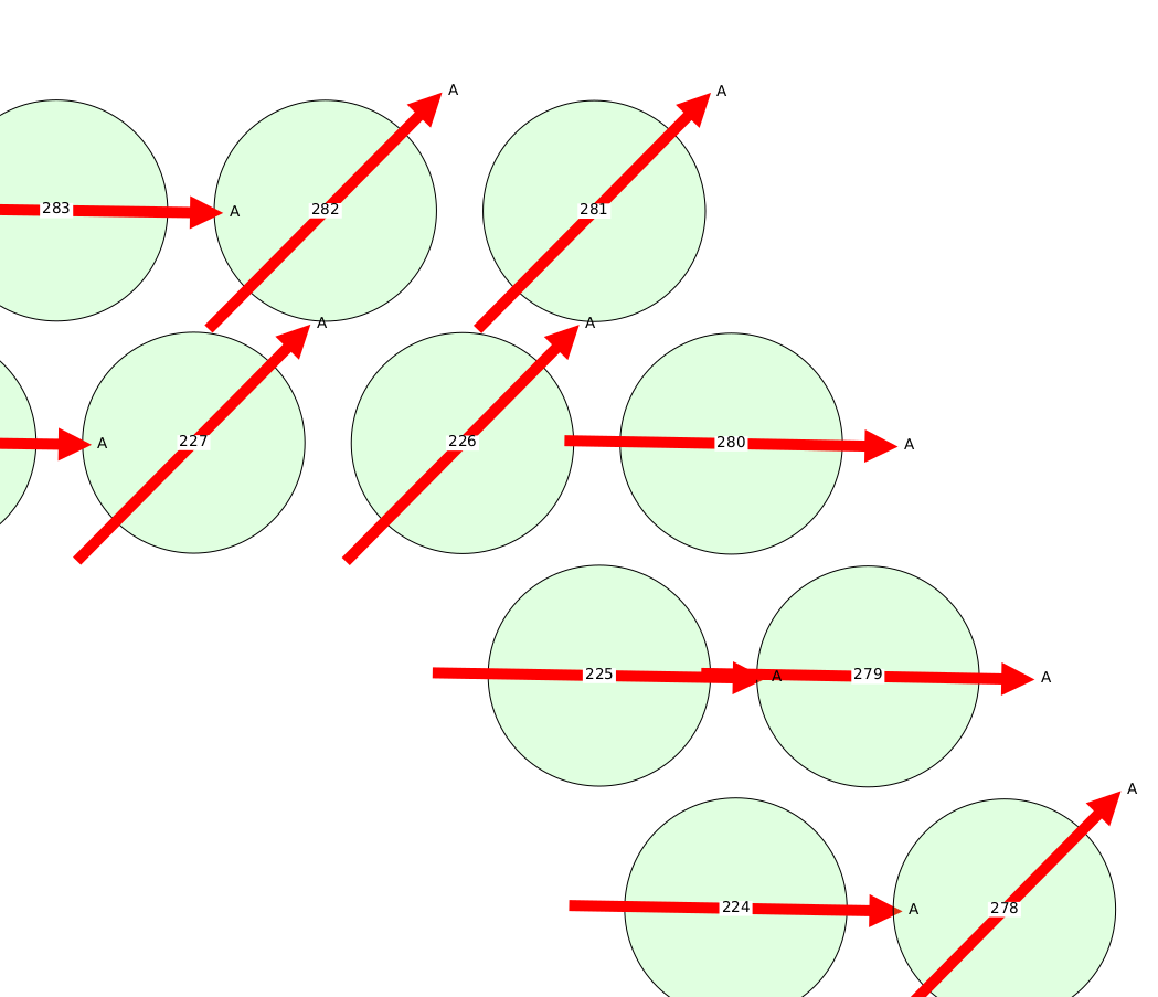
%> so_hardware_plot --hardware my_dets.toml.gz --labels
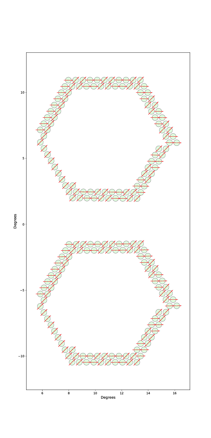
Again, the actual PDF output has “infinite” resolution. Zooming in to the above plot we can actually see the pixel labels and A/B labels on the arrows that were enabled by the –labels option: